Contents
In 2020 Armen Aghajanyan, Luke Zettlemoyer and Sonal Gupta fine-tuned RoBERTa-Large, a model with 355 million parameters, by training about 200 numbers. They chose a random 200-dimensional subspace of the full parameter space, let the optimizer move only inside it, and reached 90% of what full fine-tuning gets on MRPC, a paraphrase task[1].
Larger models needed even smaller subspaces. Two years later Tim Dettmers and colleagues fine-tuned a 65-billion-parameter model on a single 48 GB GPU, in 24 hours, and got a chatbot that GPT-4, acting as judge, rated at 99.3% of ChatGPT; the authors themselves warn that such benchmarks have wide error bars[2].
Both results say the same thing: adapting a pretrained model to a task changes very little of it. (If the transformer itself needs a refresher, the course Transformers: from scratch to production builds one.) Most of what the model knows stays put, and the change that matters can be written down with a tiny number of parameters.
Parameter-efficient fine-tuning (PEFT) is the family of methods built on that observation. This post goes through the main ones: what each adds to a transformer, written in a few lines of PyTorch, and how they compare when trained on the same task with the same budget.
What full fine-tuning costs
Fine-tuning every weight is the reference everyone compares against, and it is expensive in two ways.
The first is memory during training. With the Adam optimizer in mixed precision, every parameter costs 16 bytes: 2 for the weight in 16 bits, 2 for its gradient, and 12 for the optimizer’s state, which keeps a 32-bit master copy of the weight and two running averages[3]. For an 8-billion-parameter model that is 128 GB before a single activation is stored:
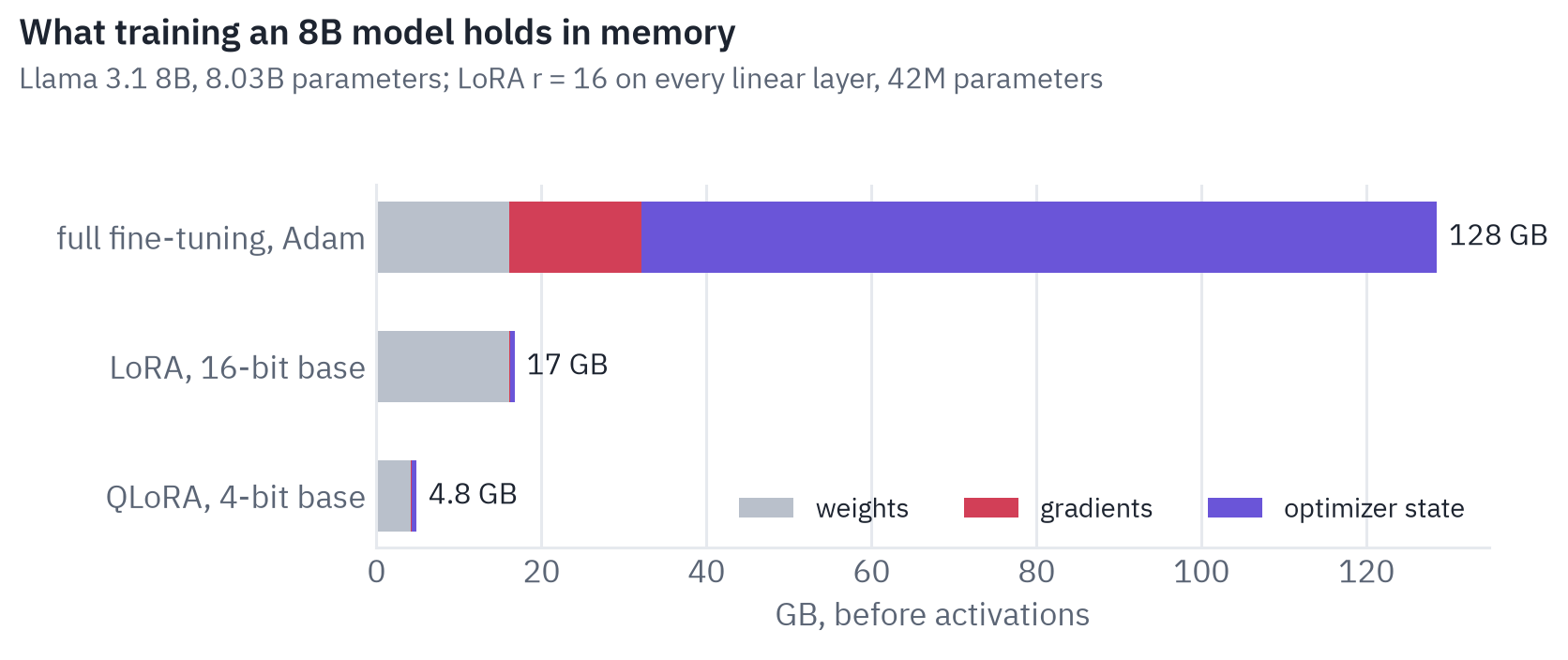
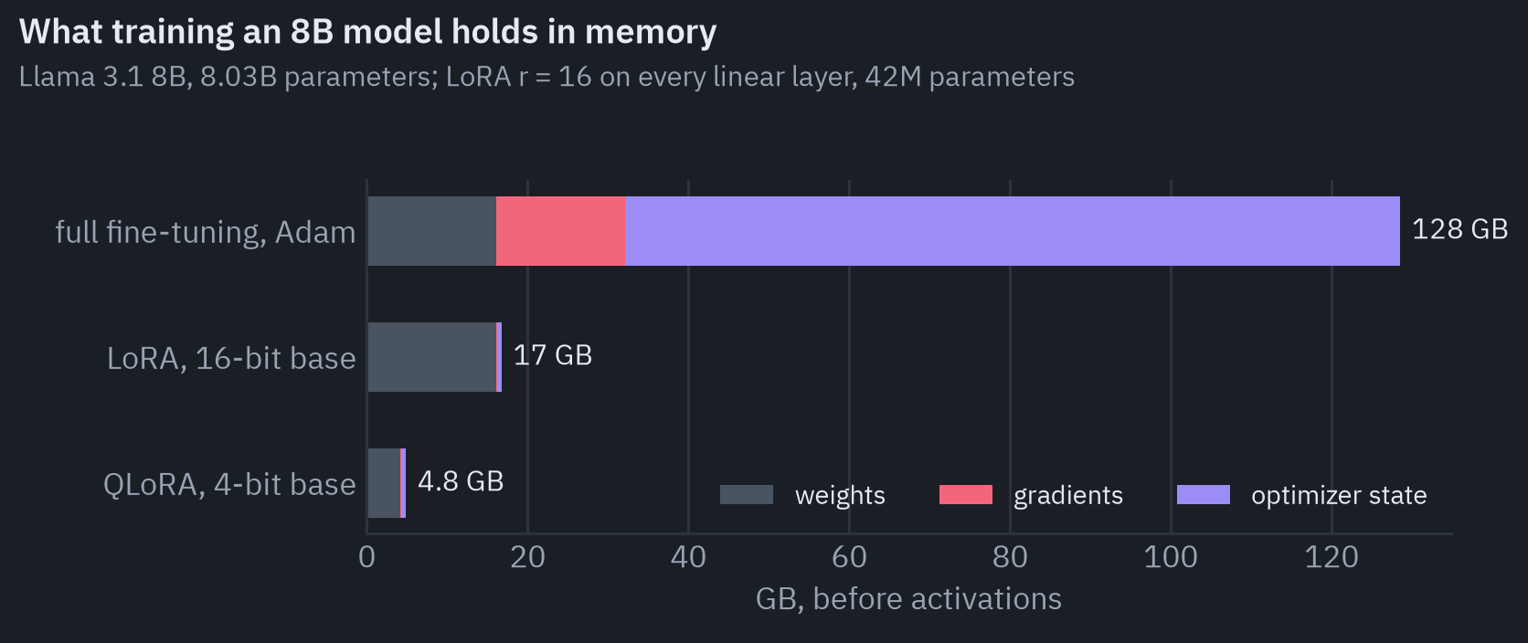
Freeze the base model and train a few million parameters instead, and the gradients and optimizer state shrink to almost nothing: what remains is the weights themselves. Store those weights in 4 bits, as QLoRA does, and the 8B model trains in a few gigabytes.
The second cost is storage. Every fully fine-tuned version is a complete copy of the model. A hundred tasks mean a hundred copies; with PEFT they mean one base model and a hundred small files, often a few megabytes each, that can be loaded, swapped and combined at will.
One idea, many places to put it
Every method below follows the same recipe. Freeze the pretrained weights. Add, or select, a small set of parameters.
Train only those, together with a task head if there is one. Junxian He and colleagues showed that most PEFT methods can be written as one operation on a hidden state[4]:
\[h \leftarrow h + \Delta h ,\]where \(h\) is some hidden representation inside the model and \(\Delta h\) is a small correction computed by the new parameters. That is the plain form; LoRA scales \(\Delta h\) by a constant, and prefix tuning, written this way, mixes \(h\) and \(\Delta h\) with a gate, \((1-\lambda) h + \lambda \Delta h\).
Key point
The methods differ in three choices: where \(\Delta h\) is added, what it is computed from, and how the function that computes it is parameterized. Keep those three questions in mind; each section below answers them for one method.
The survey by Vladislav Lialin and colleagues sorts the methods into families: those that add new parameters, those that select a subset of existing ones, and those that reparameterize the weight update[5]:
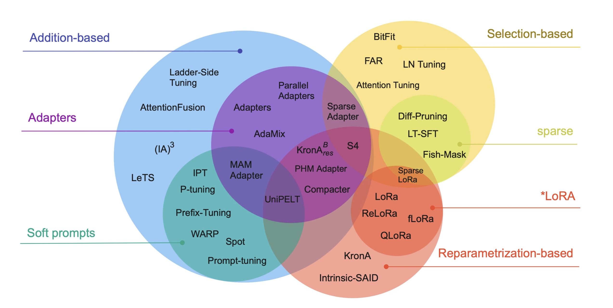
Figure 2 of Lialin, Deshpande, Yao and Rumshisky, "Scaling Down to Scale Up: A Guide to Parameter-Efficient Fine-Tuning" (version 2, 2024).
To compare the methods on equal terms, I wrote each of them in plain PyTorch, as small modules attached to a pretrained bert-base-uncased, and trained all of them on the same task: SST-2, deciding whether a sentence from a film review is positive or negative[6].
Every run uses the same 10,000 training sentences, three epochs, a learning rate chosen per method from its paper’s range, and three random seeds; every method also trains the classification head on top of BERT, about 592 thousand parameters.
The code is the code you will see below, and it ran on a Kaggle T4 (experiment.py).
Adapters
The first PEFT method for transformers, and still one of the most dependable, is the adapter of Neil Houlsby and colleagues[7]. Insert a small network into every layer, train only that network, leave everything else as it was.
The small network is a bottleneck: it projects the \(d\)-dimensional hidden state down to \(b \ll d\) numbers, applies a nonlinearity, projects back up, and adds the result to its input:
\[\text{Adapter}(h) = h + W_{\text{up}} \, \sigma\!\left(W_{\text{down}} h + b_{\text{down}}\right) + b_{\text{up}} ,\]with \(W_{\text{down}}\) of shape \(b \times d\) and \(W_{\text{up}}\) of shape \(d \times b\). In bert-base \(d = 768\); with \(b = 64\) one adapter holds 99,136 parameters.
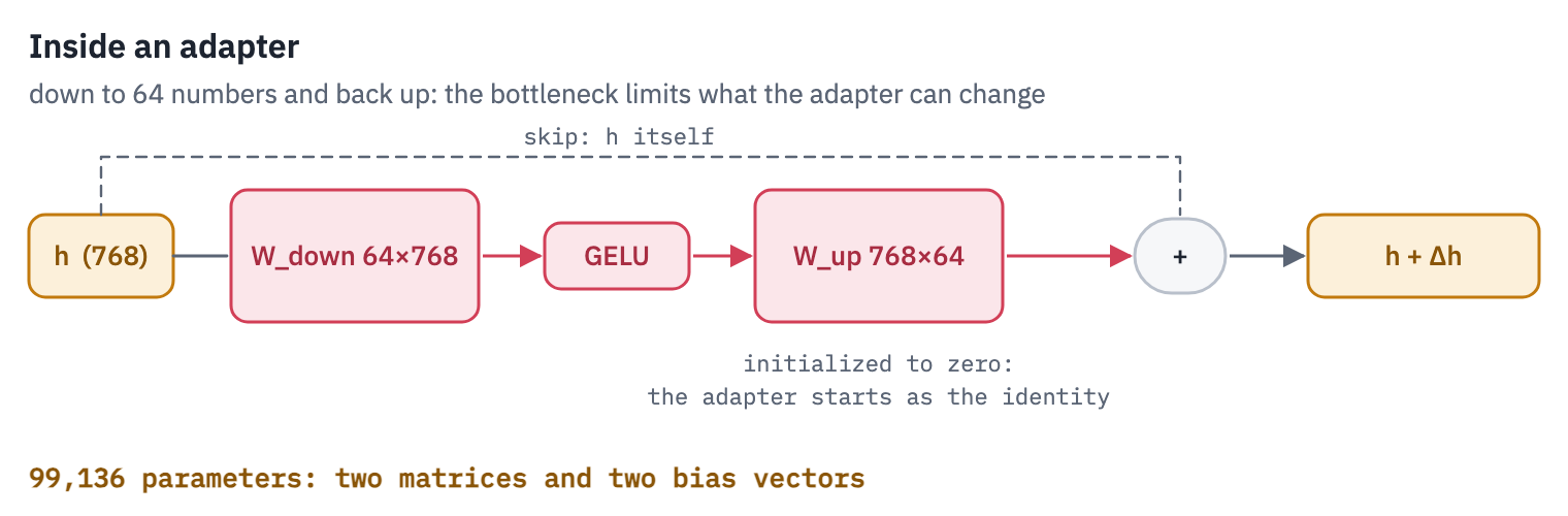
Two details decide whether this works. The first is the skip connection: the adapter computes a correction to \(h\), not a replacement for it. The second is the initialization.
If \(W_{\text{up}}\) starts at zero, the adapter’s output is exactly \(h\), so at the first step of training the model computes exactly what the pretrained model computed, and the optimizer starts from there.
Houlsby et al. initialize near the identity for this reason, and warn that “if the initialization deviates too far from the identity function, the model may fail to train.” Start from random weights instead, and every layer’s output is distorted before training even begins.
class Adapter(nn.Module):
    def __init__(self, d, bottleneck):
        super().__init__()
        self.down = nn.Linear(d, bottleneck)
        self.up = nn.Linear(bottleneck, d)
        nn.init.zeros_(self.up.weight)  # the adapter adds nothing until training moves it
        nn.init.zeros_(self.up.bias)

    def forward(self, h):
        return h + self.up(F.gelu(self.down(h)))
Where do adapters go? Houlsby et al. put two in every layer: after the projection that follows multi-head attention, and after the feed-forward block, in both cases before the residual connection and layer norm.
In Hugging Face’s BERT those projections are attention.output.dense and output.dense, and the cleanest way to insert an adapter is to replace each projection with “the projection, then the adapter”:
def add_adapters(model, bottleneck=64):
    for layer in model.bert.encoder.layer:
        # after attention and after the feed-forward block, before the residual and the layer norm
        for sub in (layer.attention.output, layer.output):
            sub.dense = nn.Sequential(sub.dense, Adapter(sub.dense.out_features, bottleneck))
Nothing else in the model changes: the residual addition and layer norm that follow dense still happen, now on the adapted output.
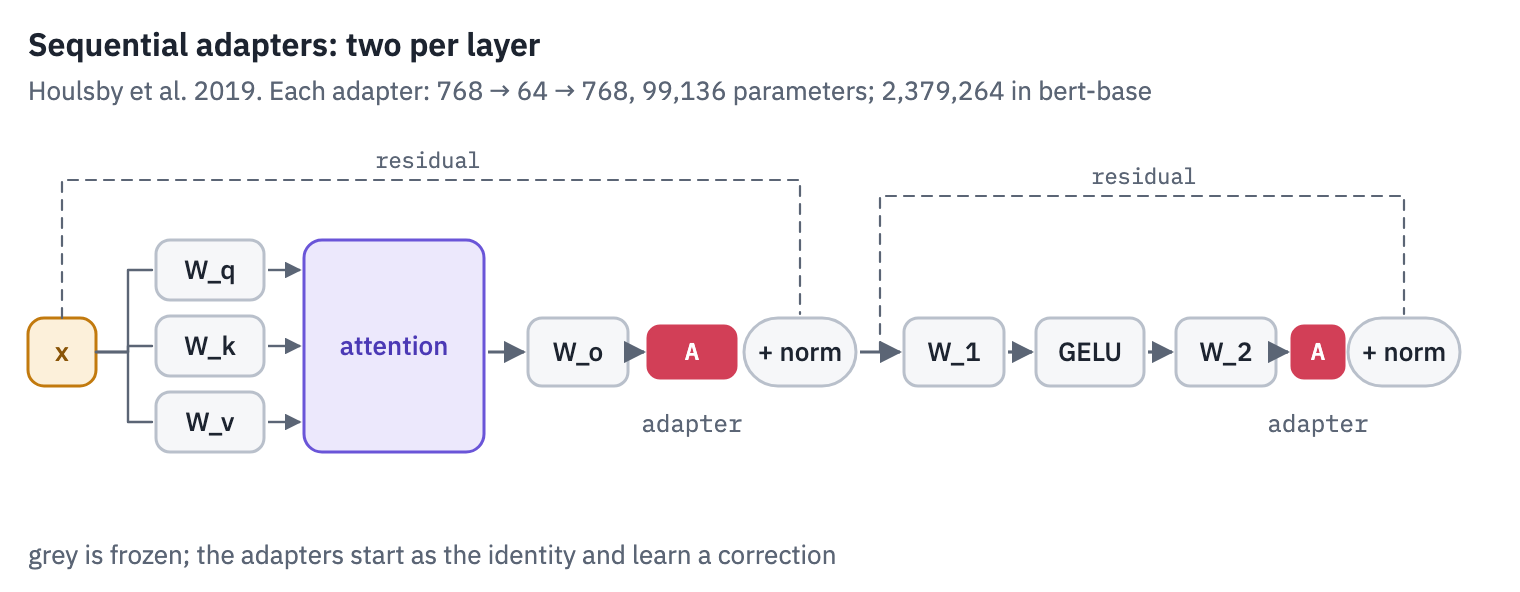
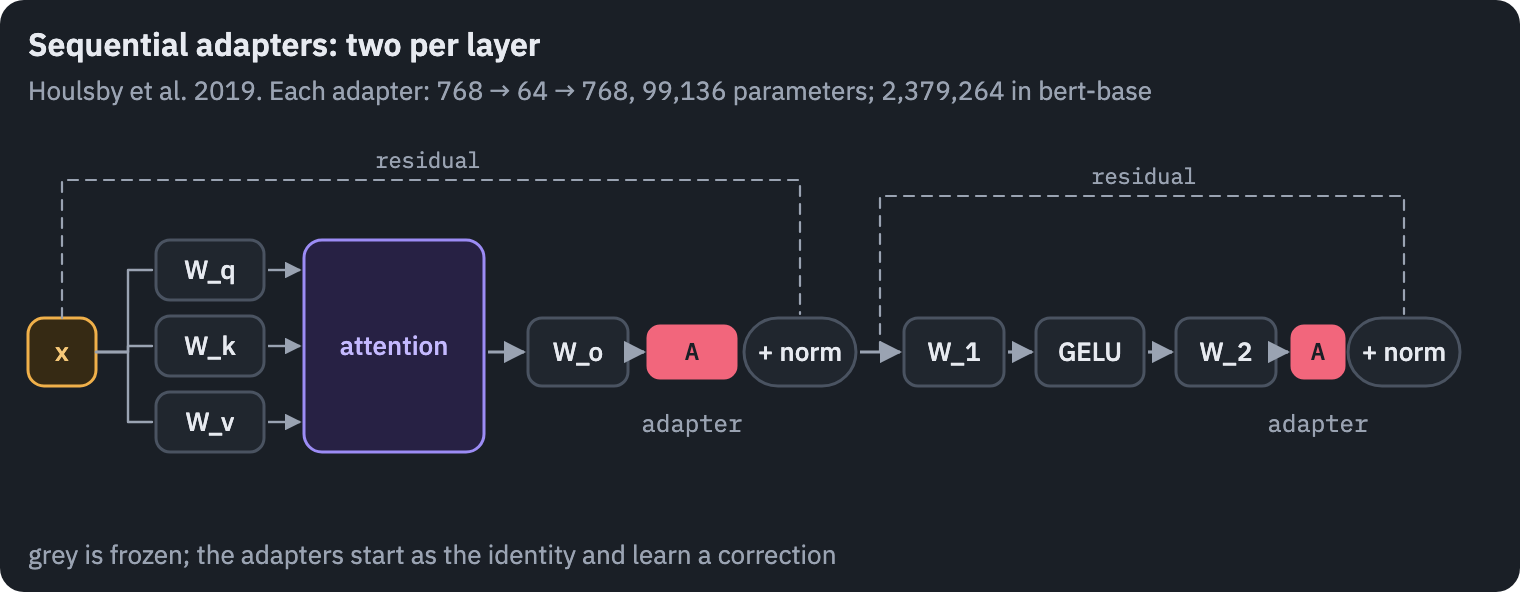
Houlsby et al. also trained the layer norms, and reported results “within 0.4% of the performance of full fine-tuning, adding only 3.6% parameters per task” on the GLUE benchmark.
Jonas Pfeiffer and colleagues later found that one adapter per layer, after the feed-forward block, performs on par “while … it requires only half the number of newly introduced adapters”[8]. Libraries long called the two layouts “Houlsby” and “Pfeiffer”.
Parallel adapters
A sequential adapter sits on the main path: every token’s hidden state must pass through it. He et al. moved it to the side. A parallel adapter reads the same input as the feed-forward block and adds its output, scaled by a constant \(s\), to the block’s output:
\[y = \text{FFN}(x) + s \cdot W_{\text{up}} \, \sigma(W_{\text{down}} x) .\]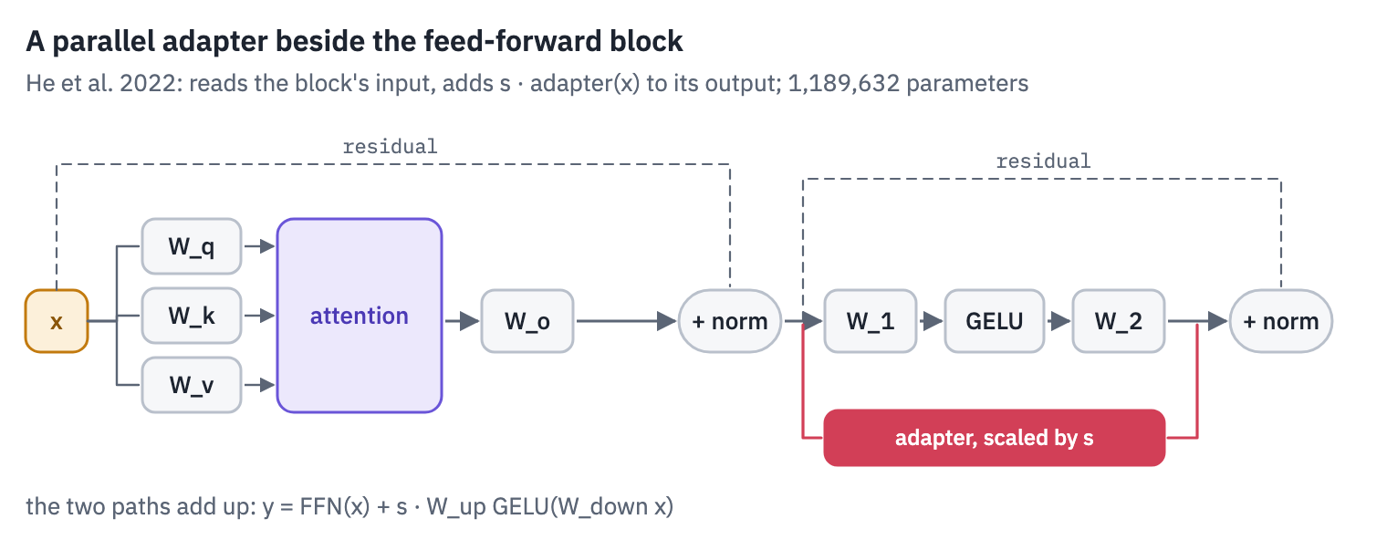
In code this means rewriting BERT’s output module, which receives both the feed-forward hidden state and the block’s input x:
class ParallelFeedForward(nn.Module):
    def __init__(self, output, bottleneck, scale=4.0):
        super().__init__()
        self.output = output  # BERT's: dense, dropout, LayerNorm(h + x)
        d = output.dense.out_features
        self.down = nn.Linear(d, bottleneck)
        self.up = nn.Linear(bottleneck, d)
        nn.init.zeros_(self.up.weight)
        nn.init.zeros_(self.up.bias)
        self.scale = scale

    def forward(self, intermediate, x):
        h = self.output.dropout(self.output.dense(intermediate))
        h = h + self.scale * self.up(F.gelu(self.down(x)))
        return self.output.LayerNorm(h + x)
The two paths no longer depend on each other, so on hardware that runs them concurrently the adapter costs less extra time. He et al. found the parallel form at least as accurate as the sequential one, especially at the feed-forward block.
The scale \(s\) is a tuned hyperparameter; they used \(s = 4\) on summarization, and AdapterHub uses 4 as its default, as do we.
LoRA
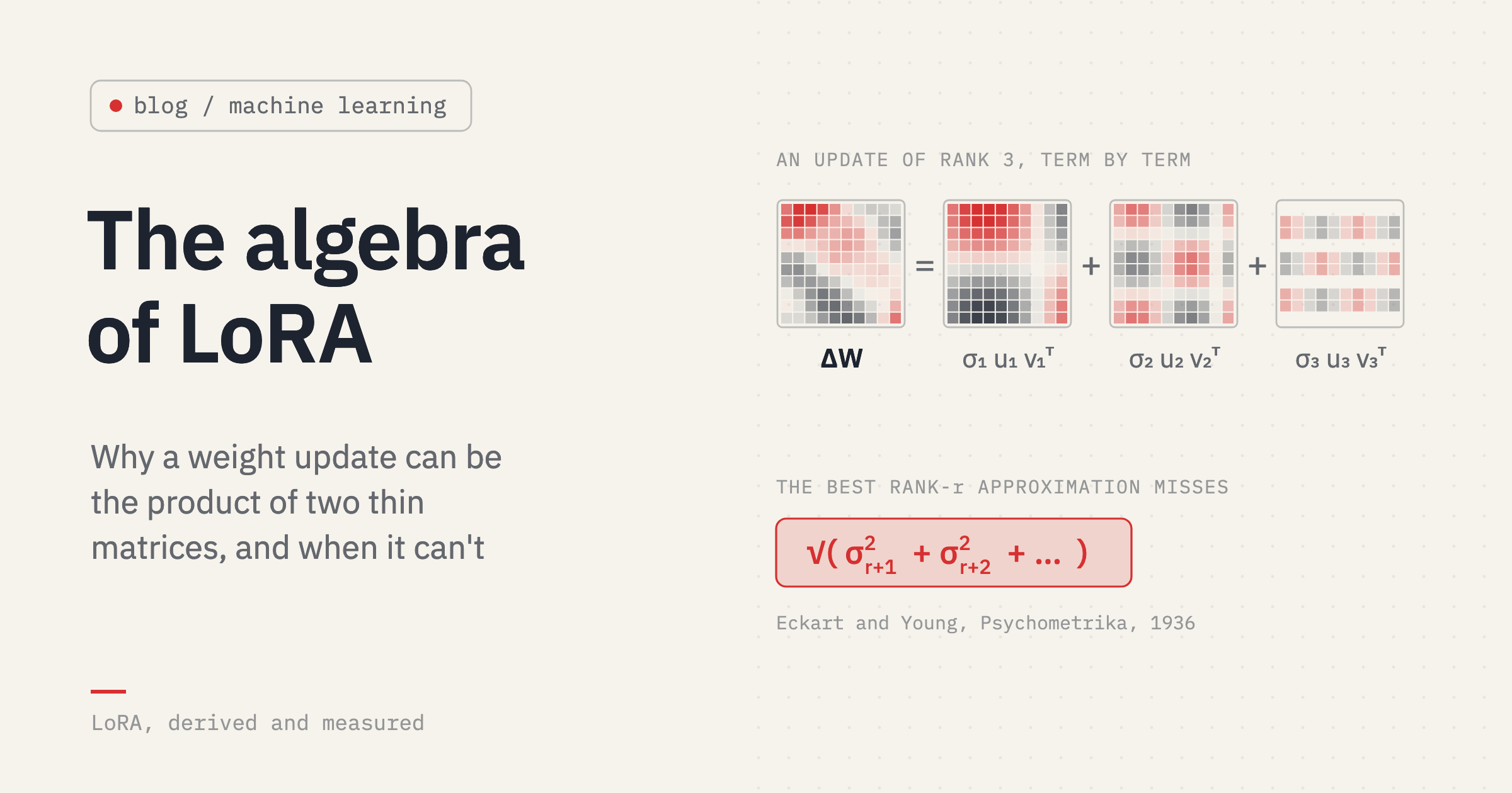
Adapters add new computations to the model. LoRA, low-rank adaptation, adds none that survive training[9]. The linear algebra behind it has a post of its own; here is what it does inside a transformer.
Its starting point is a hypothesis about the update itself. Fine-tuning changes a weight matrix \(W\) to \(W + \Delta W\). LoRA assumes \(\Delta W\) has low rank: that it can be written as the product of a tall, thin matrix and a short, wide one,
\[W' = W + \Delta W = W + \frac{\alpha}{r} B A ,\]where \(W\) is \(d_{\text{out}} \times d_{\text{in}}\) and frozen, \(B\) is \(d_{\text{out}} \times r\), \(A\) is \(r \times d_{\text{in}}\), and the rank \(r\) is small, 8 for example. The constant \(\alpha / r\) scales the update so that changing \(r\) does not require retuning the learning rate.
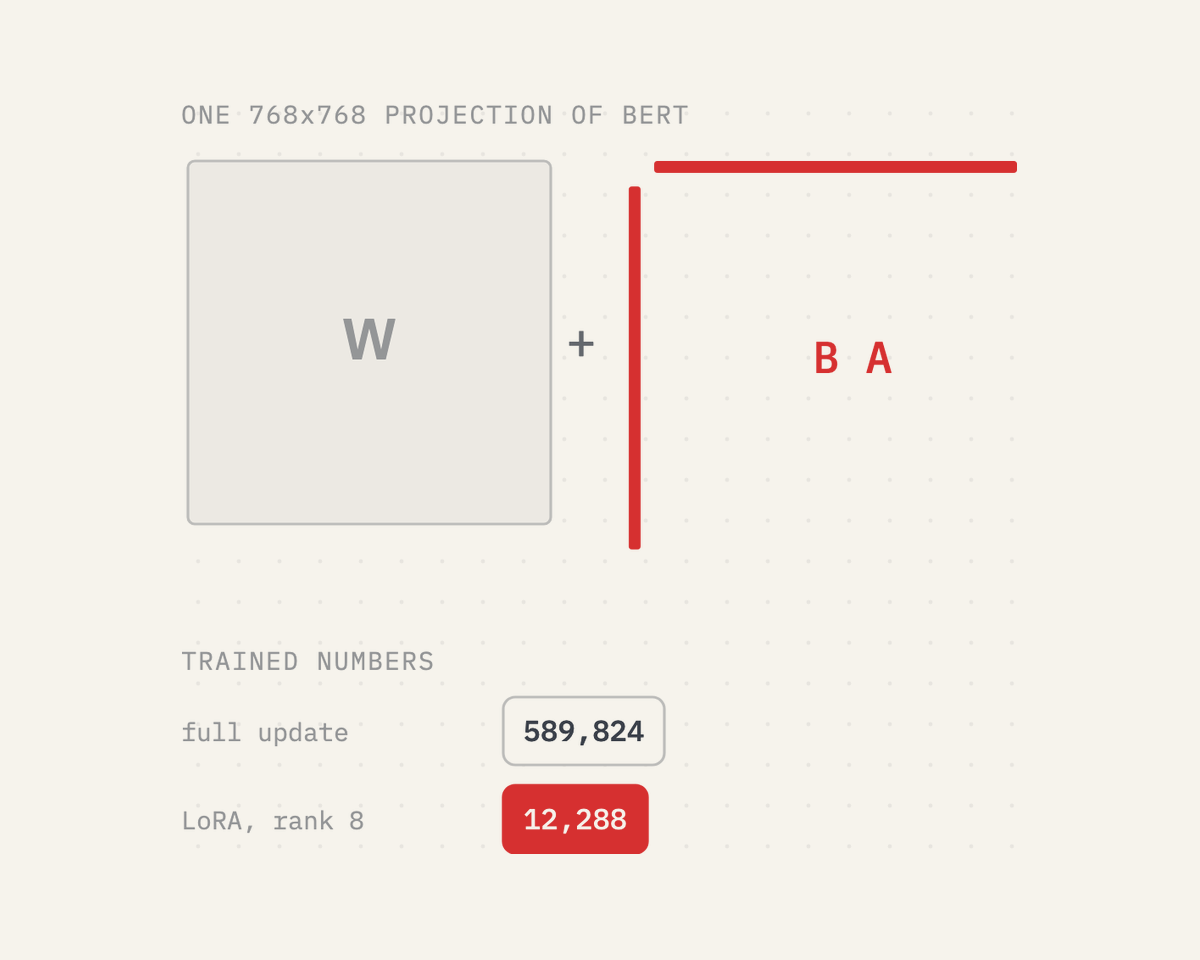
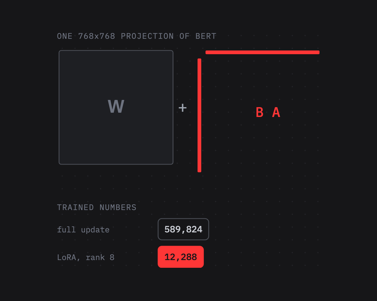
A rank-\(r\) matrix maps every input into an \(r\)-dimensional subspace first (\(A x\)) and then out again (\(B\) times that). In words: LoRA lets fine-tuning change how the layer responds along a handful of directions, and nothing else. For a \(768 \times 768\) projection, the full update has 589,824 numbers and a rank-8 one has 12,288:
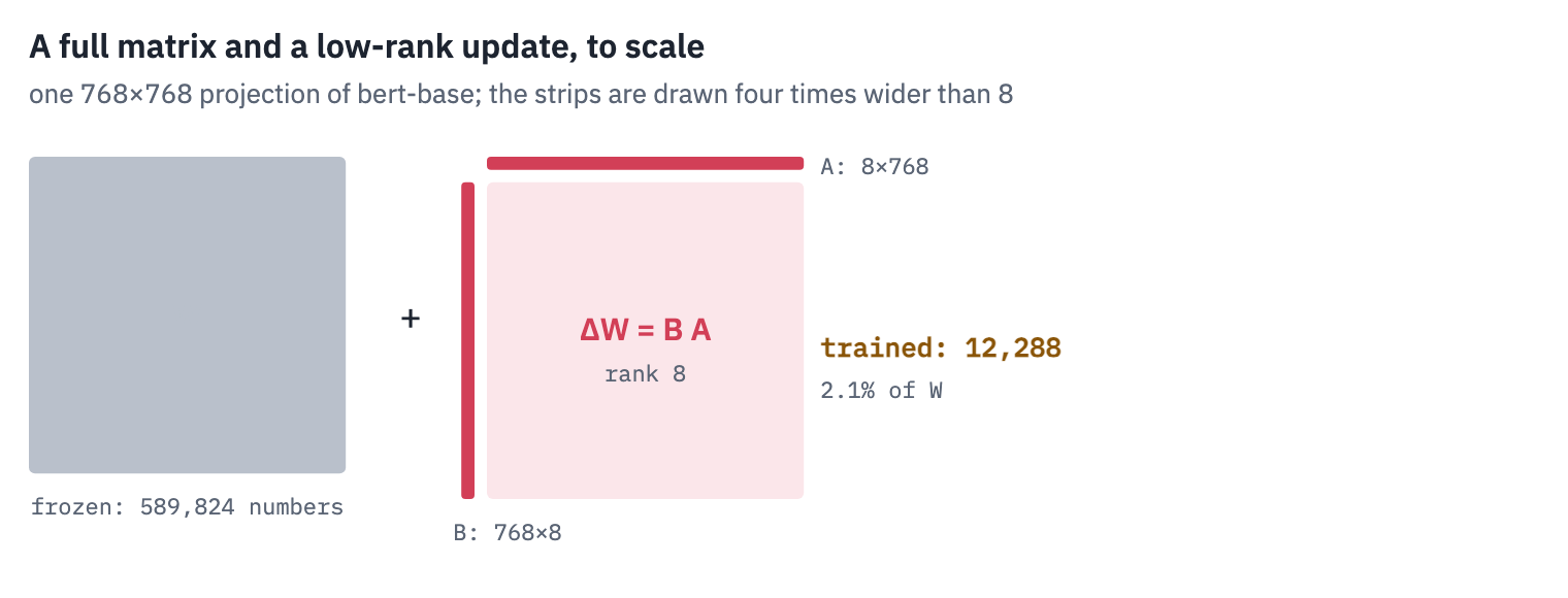
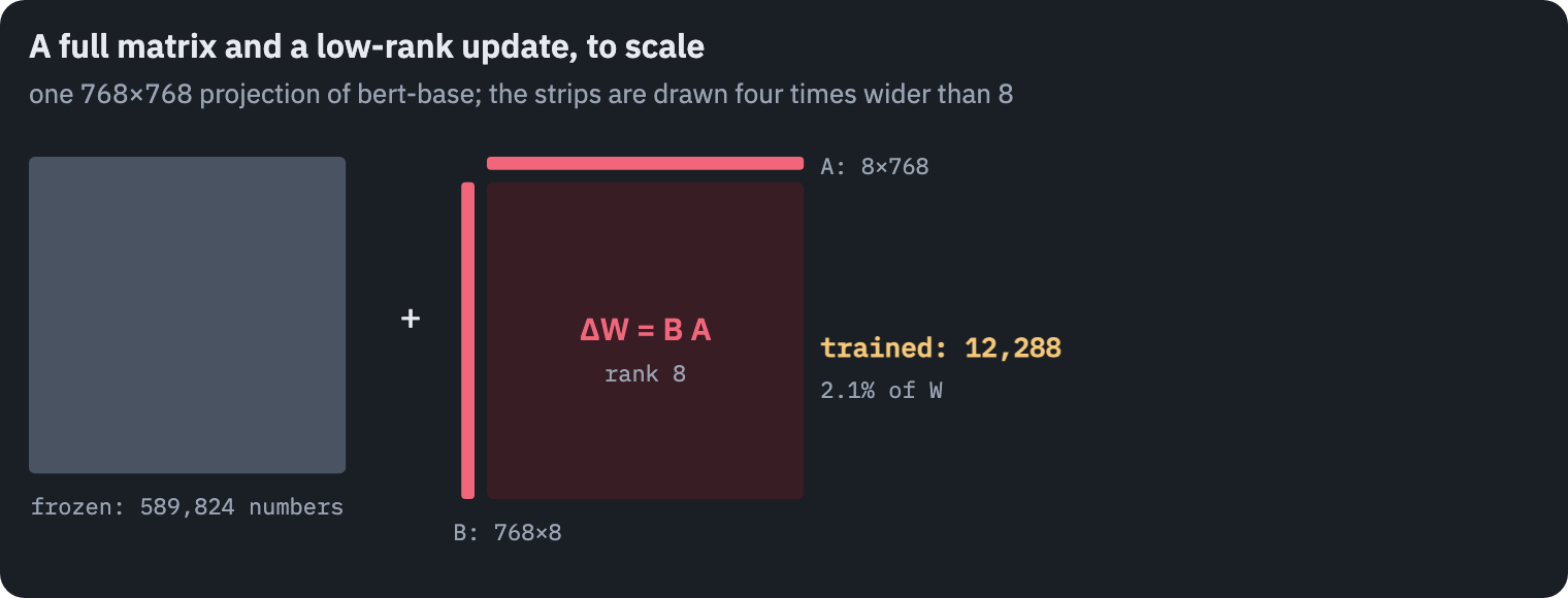
As with adapters, initialization makes the start harmless: \(A\) is random and \(B\) is zero, so \(BA = 0\) and the model begins exactly where the pretrained one was. The paper draws \(A\) from a Gaussian; Microsoft’s reference code and Hugging Face’s peft use Kaiming-uniform initialization, as below.
class LoRALinear(nn.Module):
    def __init__(self, base, r=8, alpha=16):
        super().__init__()
        self.base = base
        self.A = nn.Parameter(torch.empty(r, base.in_features))
        self.B = nn.Parameter(torch.zeros(base.out_features, r))
        nn.init.kaiming_uniform_(self.A, a=math.sqrt(5))
        self.scale = alpha / r
        self.merged = False

    def forward(self, x):
        y = self.base(x)
        if not self.merged:
            y = y + (x @ self.A.T @ self.B.T) * self.scale
        return y

    @torch.no_grad()
    def merge(self):
        self.base.weight += self.scale * self.B @ self.A
        self.merged = True
Notice the order of operations in forward: x @ A.T first, then @ B.T. The input is squeezed to \(r\) numbers before it is expanded again, so the extra cost is two thin matrix products, never a full \(d \times d\) one.
The original paper applied LoRA to the query and value projections of attention, and so do we:
def add_lora(model, r=8, alpha=16, targets=("query", "value")):
    for layer in model.bert.encoder.layer:
        attention = layer.attention.self
        for name in targets:
            setattr(attention, name, LoRALinear(getattr(attention, name), r, alpha))
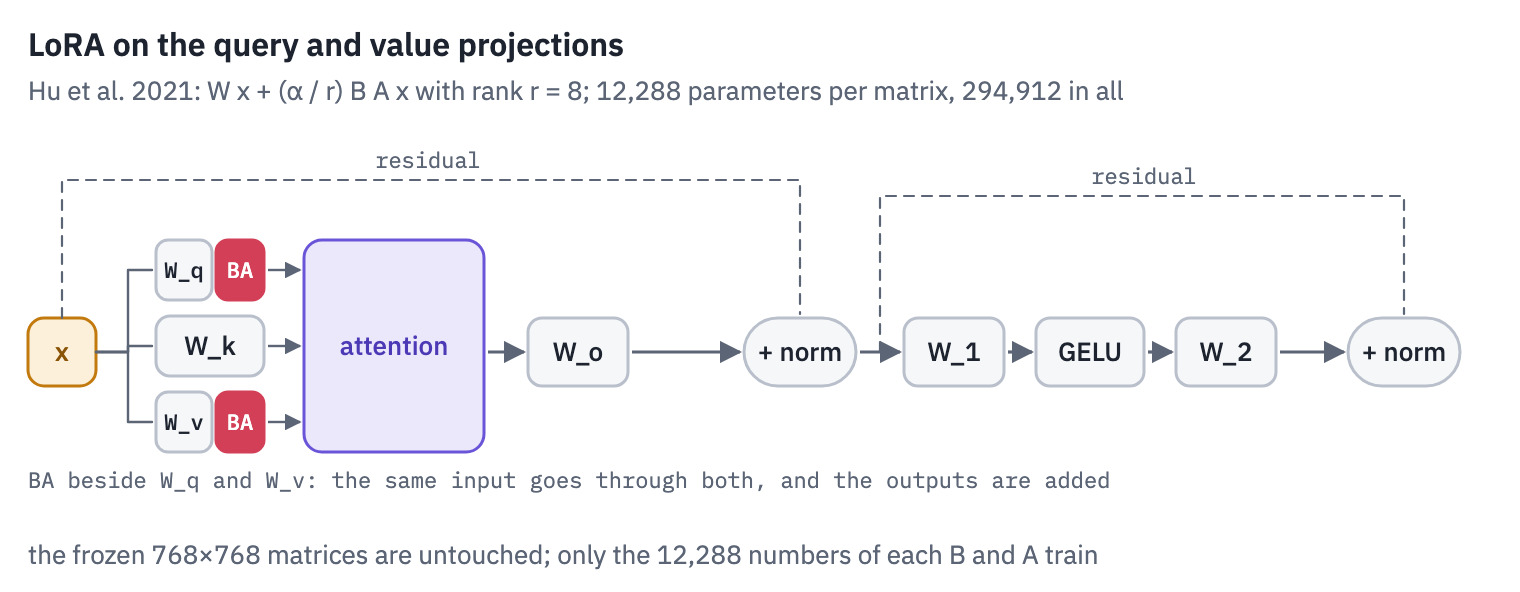
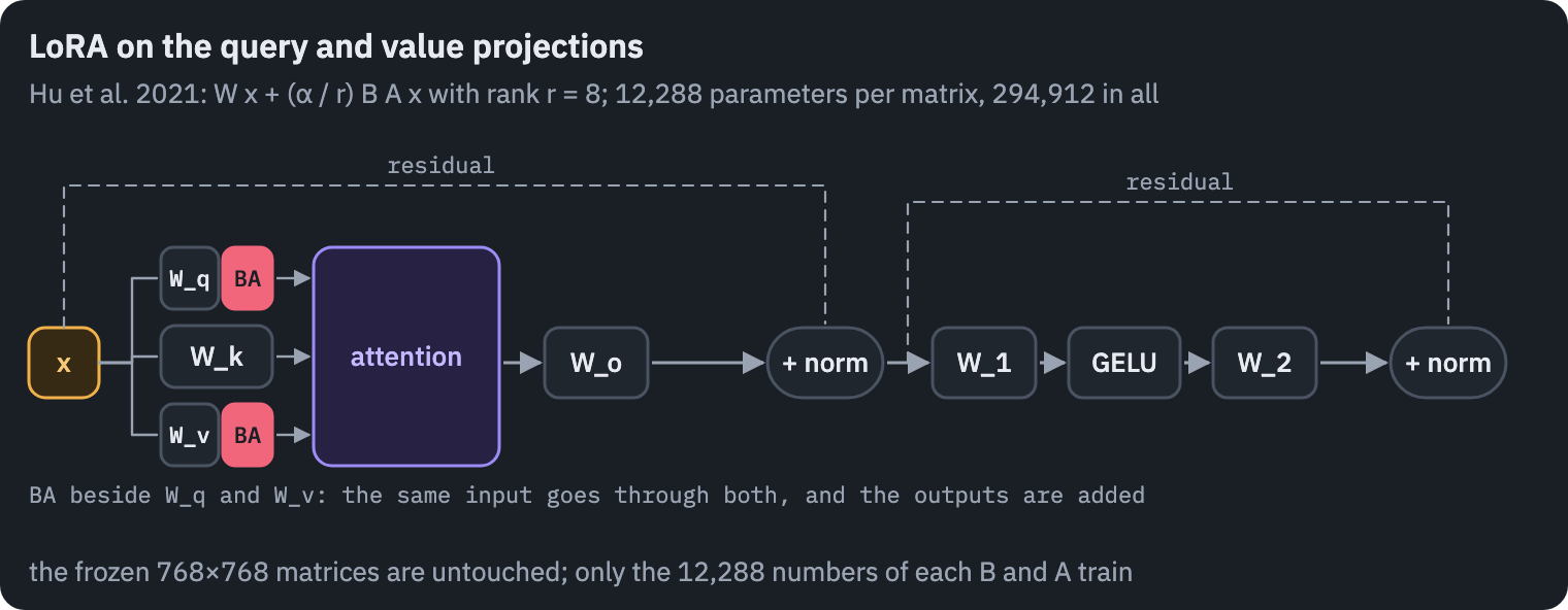
The merge method is LoRA’s best feature. After training, \(\frac{\alpha}{r} BA\) is just a matrix of the same shape as \(W\), so it can be added into \(W\) once, and the model is again an ordinary model: no extra layers, no extra latency.
In the experiment, merging changed the classifier’s outputs by at most \(2.1 \times 10^{-6}\), which is rounding error in 32-bit arithmetic.
Hu et al. report that on GPT-3 175B, LoRA cut the number of trainable parameters by 10,000 times and GPU memory during training by 3 times, from 1.2 TB to 350 GB, and that a task’s checkpoint shrank from 350 GB to 35 MB.
Is the update really low-rank?
LoRA’s hypothesis can be checked. After fully fine-tuning BERT in the experiment, I took the change in every query and value matrix, \(\Delta W = W_{\text{fine-tuned}} - W_{\text{pretrained}}\), and computed its singular values. The fraction of \(\|\Delta W\|^2\) captured by the top \(k\) singular directions tells how well a rank-\(k\) matrix could approximate the update:
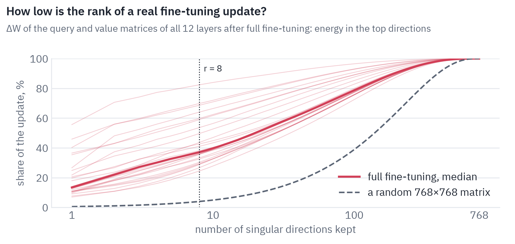
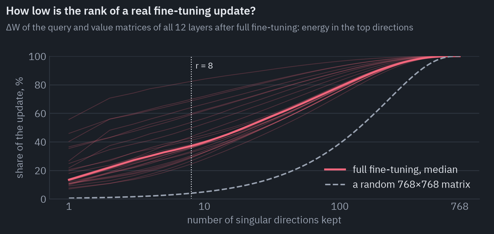
The update is far from random. Its top 8 directions hold a median of 37% of it, against 4% for a random matrix of the same size. But it is not low-rank either: holding 90% of the update takes a median of 193 directions (from 28 to 228, depending on the matrix), against 392 for random noise.
Biderman et al. found the same on a much larger scale: full fine-tuning of Llama-2-7B made changes of a rank 10 to 100 times greater than the LoRA ranks people use.
Full fine-tuning spreads its change over many directions, and LoRA works anyway: a rank-8 change turns out to be enough for the task, and the experiment below shows how close it gets.
QLoRA
QLoRA keeps LoRA’s adapters in 16 bits but stores the frozen base model in 4 bits[2]. The base weights are only read, never updated, so the quantization error enters the forward pass but not the optimizer.
Three ideas make it work: NF4, a 4-bit format whose levels are placed at the quantiles of a normal distribution, which suits trained weights; double quantization, which quantizes the scaling constants as well and saves about 0.37 bits per parameter; and paged optimizers, which use NVIDIA’s unified memory to move optimizer state to the CPU when a spike would otherwise run the GPU out of memory.
The paper also found that “LoRA on all linear transformer block layers are required to match full finetuning performance”, while the rank \(r\) mattered little.
(IA)³: rescaling instead of adding
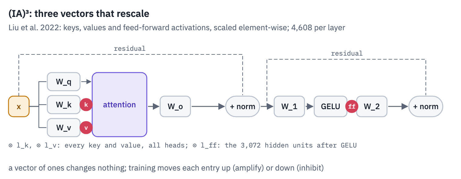
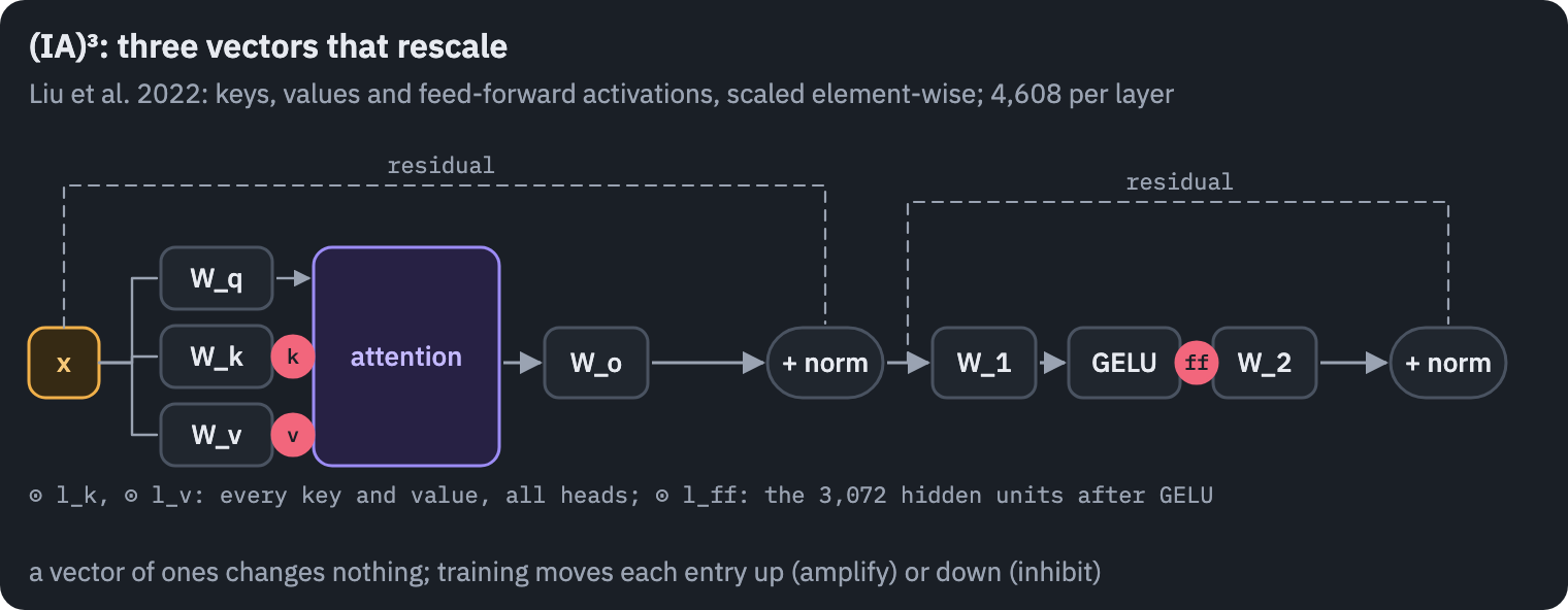
The smallest addition that can still change a model’s behaviour is a multiplication. (IA)³, “Infused Adapter by Inhibiting and Amplifying Inner Activations”, learns three vectors per layer and multiplies, element by element, the keys, the values and the hidden activations of the feed-forward block[10]:
\[\text{softmax}\!\left(\frac{Q \, (l_k \odot K)^\top}{\sqrt{d_k}}\right) (l_v \odot V), \qquad (l_{ff} \odot \gamma(W_1 x)) \, W_2 .\]Each vector starts at ones, which multiplies by one and changes nothing. Training moves each entry above one, amplifying a feature, or below, inhibiting it.
class Rescale(nn.Module):
    def __init__(self, module, size):
        super().__init__()
        self.module = module
        self.scale = nn.Parameter(torch.ones(size))

    def forward(self, x):
        return self.module(x) * self.scale


def add_ia3(model):
    for layer in model.bert.encoder.layer:
        attention = layer.attention.self
        attention.key = Rescale(attention.key, attention.key.out_features)  # l_k
        attention.value = Rescale(attention.value, attention.value.out_features)  # l_v
        hidden = layer.intermediate.dense.out_features
        layer.intermediate = Rescale(layer.intermediate, hidden)  # l_ff, after GELU
In bert-base that is \(768 + 768 + 3072 = 4{,}608\) numbers per layer, 55,296 in all, about 0.05% of the model. Like LoRA, the vectors can be folded into the weights after training, since \(l \odot (W x) = (l \odot W) x\).
BitFit: train the biases
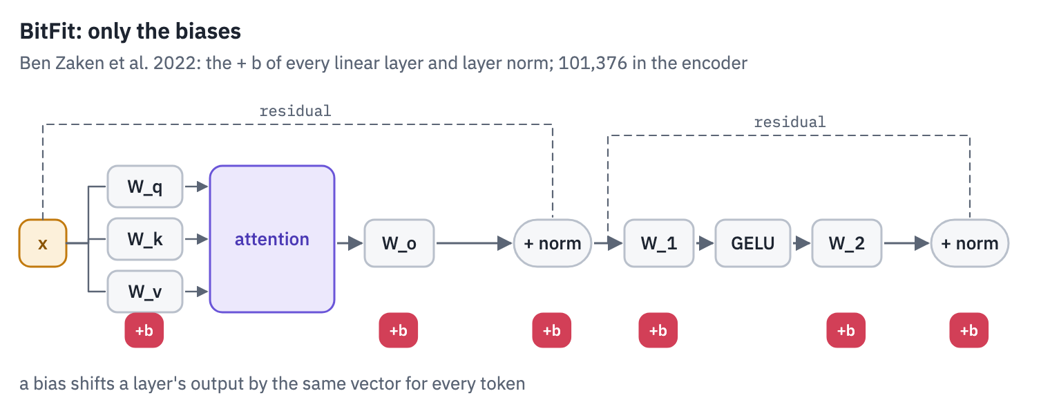
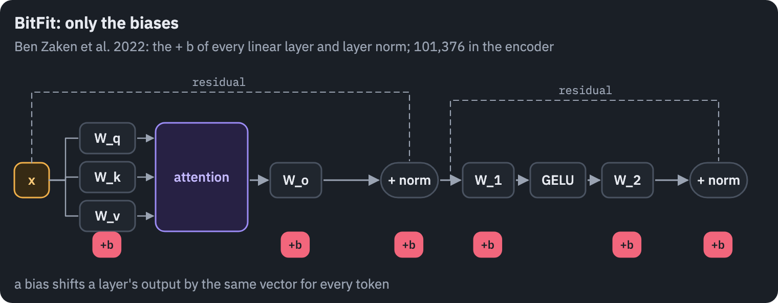
BitFit adds nothing. It trains a subset of what is already there: the bias vectors of every linear layer and layer norm[11]. A bias shifts a layer’s output by the same vector for every token, so BitFit can move representations but cannot change how a layer mixes its inputs.
def bitfit(model):
    for name, p in model.bert.named_parameters():
        if name.endswith("bias"):
            p.requires_grad = True
There are 101,376 bias numbers in bert-base’s encoder, plus 768 in the embedding layer norm, under 0.1% of the model.
Prompt tuning and prefix tuning
The methods so far change what a layer computes. The next two change what it sees.
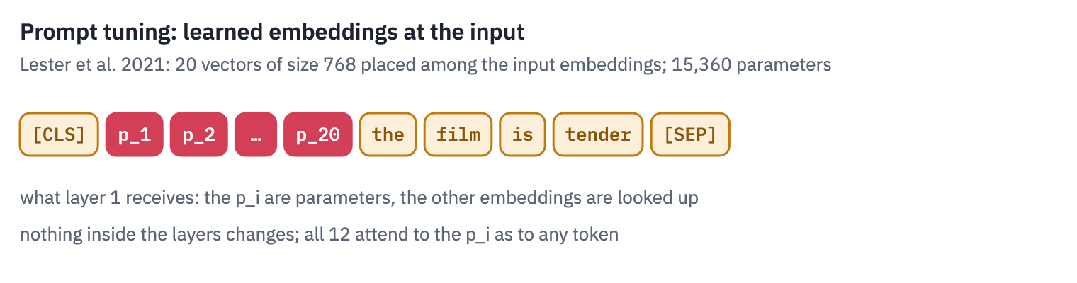
Prompt tuning prepends learned vectors to the input[12]. A text prompt is a sequence of token embeddings looked up in a table. A soft prompt is a sequence of embeddings that are parameters: the optimizer can place them anywhere in embedding space, not only at the positions of real words.
class SoftPrompt(nn.Module):
    def __init__(self, model, length=20):
        super().__init__()
        self.model = model
        vocabulary = model.get_input_embeddings().weight
        # begin from the embeddings of real words
        start = torch.randint(1000, vocabulary.shape[0], (length,))
        self.prompt = nn.Parameter(vocabulary[start].detach().clone())

    def forward(self, input_ids, attention_mask, labels=None):
        embeds = self.model.get_input_embeddings()(input_ids)
        prompt = self.prompt.expand(input_ids.shape[0], -1, -1)
        embeds = torch.cat([embeds[:, :1], prompt, embeds[:, 1:]], dim=1)
        mask = torch.cat([attention_mask[:, :1].expand(-1, prompt.shape[1]), attention_mask], dim=1)
        return self.model(inputs_embeds=embeds, attention_mask=mask, labels=labels)
The prompt goes after [CLS] because BERT classifies from the first position. Twenty vectors of 768 numbers are 15,360 parameters, by far the fewest of any method here, and the result shows it: in the experiment below it reached 85.5% on average, no better than training the classification head alone (85.9%).
Lester et al. found the same pattern on a much larger scale. With T5 models of up to 11 billion parameters, prompt tuning trailed full fine-tuning on small models and caught up with it only as models grew past a few billion parameters.
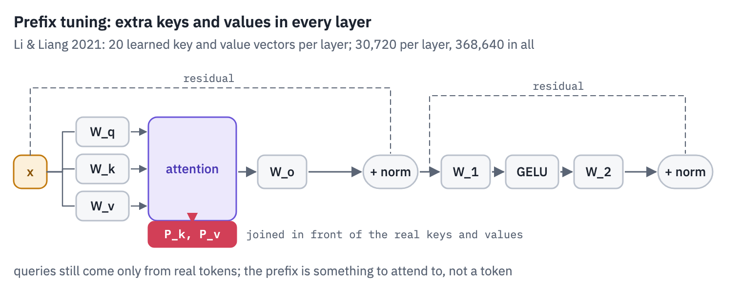
Prefix tuning gives the learned vectors more reach[13]. Instead of input embeddings, it learns keys and values for every layer: each layer’s attention sees \(p\) extra key-value pairs, as if \(p\) invisible tokens preceded the input at that depth:
\[\text{head} = \text{softmax}\!\left(\frac{Q \, [P_k ; K]^\top}{\sqrt{d_k}}\right) [P_v ; V] ,\]where \([\,\cdot\,;\,\cdot\,]\) joins the learned rows \(P_k, P_v\) in front of the real keys and values. Queries still come only from the real tokens.
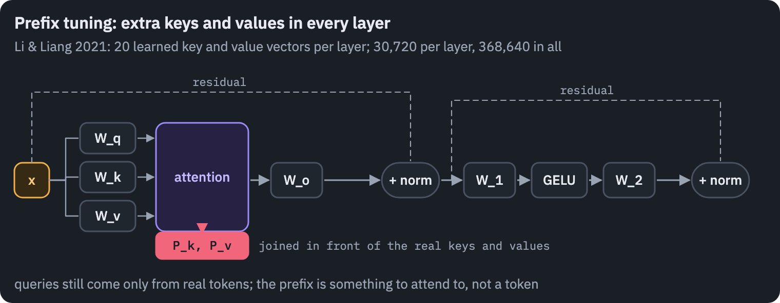
This is a change to attention itself, and recent versions of transformers let you register your own attention function under a name. The whole of prefix tuning is one such function, which joins the layer’s prefix in front of its keys and values and then calls the standard implementation:
def prefix_attention(module, query, key, value, attention_mask, **kwargs):
    batch = key.shape[0]
    # (batch, heads, length, head_dim), in the precision of the keys
    prefix_k = module.prefix_key.expand(batch, -1, -1, -1).to(key.dtype)
    prefix_v = module.prefix_value.expand(batch, -1, -1, -1).to(value.dtype)
    key = torch.cat([prefix_k, key], dim=2)
    value = torch.cat([prefix_v, value], dim=2)
    # the mask is boolean, True where attention is allowed: the prefix is always visible
    if attention_mask is not None:
        visible = attention_mask.new_ones(*attention_mask.shape[:-1], prefix_k.shape[2])
        attention_mask = torch.cat([visible, attention_mask], dim=-1)
    return sdpa_attention_forward(module, query, key, value, attention_mask, **kwargs)


AttentionInterface.register("prefix", prefix_attention)
AttentionMaskInterface.register("prefix", sdpa_mask)


def add_prefix(model, length=20):
    model.set_attn_implementation("prefix")
    for layer in model.bert.encoder.layer:
        attention = layer.attention.self
        shape = (1, attention.num_attention_heads, length, attention.attention_head_size)
        attention.prefix_key = nn.Parameter(torch.randn(shape) * 0.02)
        attention.prefix_value = nn.Parameter(torch.randn(shape) * 0.02)
Trap
A custom attention function also needs a rule for building the padding mask, registered with AttentionMaskInterface as above. Without it the model silently passes no mask at all.
Li and Liang trained the prefix through a small MLP rather than directly, because optimizing the raw vectors was unstable; after training the MLP is thrown away and only the prefix kept.
Compacter: adapters built from Kronecker products
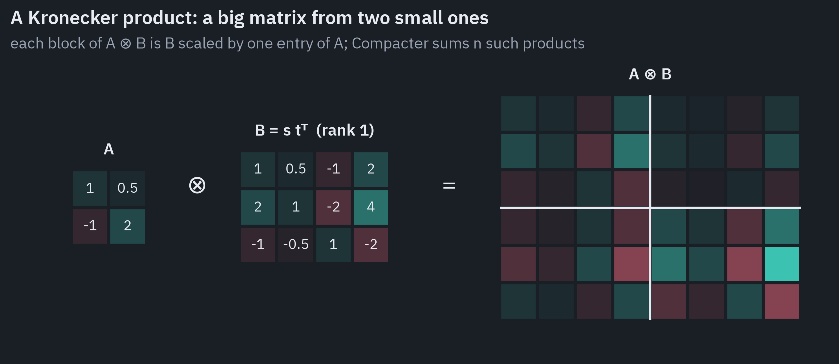
Compacter shrinks the adapter’s two matrices further[14]. It builds each of them as a sum of Kronecker products. The Kronecker product \(A \otimes B\) of an \(m \times n\) matrix and a \(p \times q\) one is an \(mp \times nq\) matrix made of blocks: block \((i, j)\) is \(B\) multiplied by the entry \(a_{ij}\).
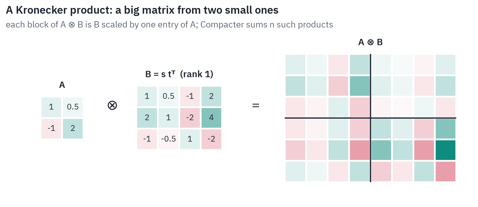
Compacter writes each adapter matrix as
\[W = \sum_{i=1}^{n} A_i \otimes B_i ,\]with two twists that make it small. The \(n \times n\) matrices \(A_i\) are shared by every adapter in the model; they capture structure common to all layers. And each \(B_i\) has rank one, \(B_i = s_i t_i^\top\), so it costs only the length of two vectors.
With \(n = 4\), the down-projection of a 48-unit adapter in bert-base needs 816 numbers instead of 36,864. On T5-base the paper reports GLUE results on par with full fine-tuning while training 0.073% of the parameters, and 0.047% for Compacter++, which keeps only the adapter after the feed-forward block.
class PHMLinear(nn.Module):
    def __init__(self, shared, d_in, d_out, zero=False):
        super().__init__()
        n = shared.shape[0]
        self.shared = shared  # (n, n, n): A_1 ... A_n, the same tensor in every layer
        if zero:
            self.s = nn.Parameter(torch.zeros(n, d_out // n, 1))
        else:
            self.s = nn.Parameter(torch.randn(n, d_out // n, 1) * 0.1)
        self.t = nn.Parameter(torch.randn(n, 1, d_in // n) * 0.1)
        self.bias = nn.Parameter(torch.zeros(d_out))

    def weight(self):
        B = self.s @ self.t  # (n, d_out / n, d_in / n), each of rank one
        return sum(torch.kron(self.shared[i], B[i]) for i in range(len(B)))

    def forward(self, x):
        return F.linear(x, self.weight(), self.bias)
The adapter itself is unchanged; only its two nn.Linear layers become PHMLinear, with the up-projection’s \(s_i\) starting at zero so that, once again, the adapter starts as the identity.
The same task, ten ways
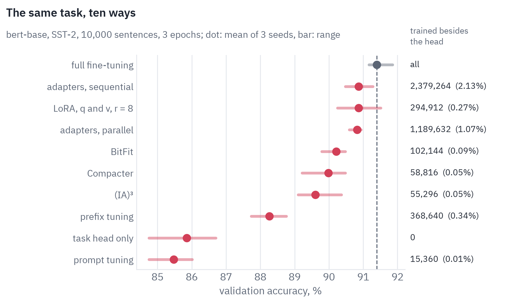
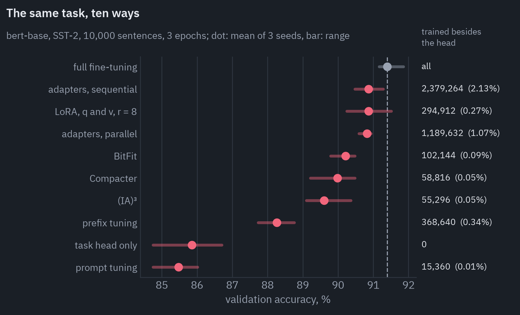
Here is how the methods compare on SST-2, against the number of parameters each trains besides the classification head:
| method | trained besides the head | accuracy, % (3 seeds) | time per run | peak GPU memory |
|---|---|---|---|---|
| full fine-tuning | all 109M | 91.4 (91.2–91.9) | 97 s | 2.28 GiB |
| LoRA, q and v, r = 8 | 294,912 (0.27%) | 90.9 (90.3–91.5) | 48 s | 1.26 GiB |
| adapters, sequential | 2,379,264 (2.13%) | 90.9 (90.5–91.3) | 50 s | 1.28 GiB |
| adapters, parallel | 1,189,632 (1.07%) | 90.8 (90.6–90.9) | 45 s | 1.19 GiB |
| BitFit | 102,144 (0.09%) | 90.2 (89.8–90.5) | 44 s | 1.20 GiB |
| Compacter | 58,816 (0.05%) | 90.0 (89.2–90.5) | 110 s | 1.25 GiB |
| (IA)³ | 55,296 (0.05%) | 89.6 (89.1–90.4) | 55 s | 1.44 GiB |
| prefix tuning | 368,640 (0.34%) | 88.3 (87.7–88.8) | 44 s | 1.22 GiB |
| task head only | none | 85.9 (84.7–86.7) | 22 s | 0.53 GiB |
| prompt tuning | 15,360 (0.01%) | 85.5 (84.7–86.0) | 60 s | 1.35 GiB |
Three methods come within half a point of full fine-tuning: LoRA with 0.27% of the model’s parameters, and adapters in both arrangements with 1 to 2%.
BitFit, Compacter and (IA)³, each with less than a tenth of a percent, lose about one to two points. Prefix tuning loses three. Prompt tuning learned nothing that the task head alone did not, as Lester et al.’s results predict for a model this small.
The memory column shows a smaller saving than the chart at the top of this post, because bert-base is small: at 110 million parameters the activations of a batch take about as much memory as the optimizer state, and the activations remain.
Still, every method cut the peak memory of full fine-tuning by a third to a half, and most of them halved the time. Compacter is the exception in time: it rebuilds its matrices from Kronecker products at every step, which the other methods do not have to do.
A caution about reading too much into the ranking. This is one model, one task and three seeds, with learning rates taken from the papers rather than tuned for each method, and the ranges of the top four overlap. What the table shows reliably is the shape of the trade-off, not a winner.
In practice
Nobody writes these modules by hand for production. Hugging Face’s peft library implements most of them behind one interface:
from peft import LoraConfig, get_peft_model
from transformers import AutoModelForSequenceClassification

model = AutoModelForSequenceClassification.from_pretrained("bert-base-uncased", num_labels=2)
config = LoraConfig(
    r=8, lora_alpha=16, target_modules=["query", "value"], lora_dropout=0.1, task_type="SEQ_CLS"
)
model = get_peft_model(model, config)
model.print_trainable_parameters()
# ... train as usual, then:
model = model.merge_and_unload()  # LoRA folded into the weights; an ordinary model again
The adapters library from AdapterHub, which replaced the older adapter-transformers, does the same for bottleneck adapters, prefix tuning, Compacter and their combinations:
from adapters import AutoAdapterModel

model = AutoAdapterModel.from_pretrained("bert-base-uncased")
# "seq_bn": one adapter per layer; "double_seq_bn": Houlsby's two; also "par_bn", "compacter", ...
model.add_adapter("sst2", config="seq_bn")
model.add_classification_head("sst2", num_labels=2)
model.train_adapter("sst2")  # freezes everything but the adapter and the head
# ... train, then keep only the adapter:
model.save_adapter("./sst2_adapter", "sst2")
A few things are worth knowing before you start:
- Where to put LoRA. The original paper adapted the query and value projections. QLoRA found that adapting every linear layer of the blocks is what closes the gap with full fine-tuning, and
peftacceptstarget_modules="all-linear"for that. - What LoRA does not learn. Dan Biderman and colleagues compared LoRA with full fine-tuning of Llama-2-7B on code and mathematics: in the usual low-rank settings LoRA learned less of the new domain and forgot less of the old one, and full fine-tuning made weight changes of “a rank that is 10-100× greater than typical LoRA configurations”[15]. For instruction tuning on a narrow task the trade is usually welcome; for teaching a model a new field through continued pre-training, it may not be.
- Many adapters, one model. Because adapters are small and the base is shared, one server can hold many of them at once and apply a different one to each request. S-LoRA serves thousands of LoRA adapters on a single GPU[16], and vLLM applies adapters per request.
References
- Aghajanyan, A., Zettlemoyer, L., & Gupta, S. (2021). Intrinsic dimensionality explains the effectiveness of language model fine-tuning. ACL-IJCNLP. ↩
- Dettmers, T., Pagnoni, A., Holtzman, A., & Zettlemoyer, L. (2023). QLoRA: efficient finetuning of quantized LLMs. NeurIPS. ↩
- Rajbhandari, S., Rasley, J., Ruwase, O., & He, Y. (2020). ZeRO: memory optimizations toward training trillion parameter models. SC20. ↩
- He, J., Zhou, C., Ma, X., Berg-Kirkpatrick, T., & Neubig, G. (2022). Towards a unified view of parameter-efficient transfer learning. ICLR. ↩
- Lialin, V., Deshpande, V., Yao, X., & Rumshisky, A. (2023). Scaling down to scale up: a guide to parameter-efficient fine-tuning. arXiv:2303.15647. ↩
- Socher, R., et al. (2013). Recursive deep models for semantic compositionality over a sentiment treebank. EMNLP. ↩
- Houlsby, N., et al. (2019). Parameter-efficient transfer learning for NLP. ICML. ↩
- Pfeiffer, J., Kamath, A., Rücklé, A., Cho, K., & Gurevych, I. (2021). AdapterFusion: non-destructive task composition for transfer learning. EACL. ↩
- Hu, E. J., et al. (2021). LoRA: low-rank adaptation of large language models. ICLR 2022. ↩
- Liu, H., et al. (2022). Few-shot parameter-efficient fine-tuning is better and cheaper than in-context learning. NeurIPS. ↩
- Ben Zaken, E., Ravfogel, S., & Goldberg, Y. (2022). BitFit: simple parameter-efficient fine-tuning for transformer-based masked language-models. ACL. ↩
- Lester, B., Al-Rfou, R., & Constant, N. (2021). The power of scale for parameter-efficient prompt tuning. EMNLP. ↩
- Li, X. L., & Liang, P. (2021). Prefix-tuning: optimizing continuous prompts for generation. ACL-IJCNLP. ↩
- Karimi Mahabadi, R., Henderson, J., & Ruder, S. (2021). Compacter: efficient low-rank hypercomplex adapter layers. NeurIPS. ↩
- Biderman, D., et al. (2024). LoRA learns less and forgets less. TMLR. ↩
- Sheng, Y., et al. (2023). S-LoRA: serving thousands of concurrent LoRA adapters. MLSys 2024. ↩
- Libraries: Hugging Face peft, AdapterHub adapters, vLLM LoRA adapters.
The experiment, with every method above, and the figures: articles/adapters.
Reference and BibTeX
Koroleva, E. (2025, April 17). Parameter-efficient fine-tuning in PyTorch: adapters, LoRA and the rest. Eva Koroleva's blog. https://blog.korolevalab.com/blog/2025/adapters/
@misc{koroleva2025adapters,
  author       = {Koroleva, Eva},
  title        = {{Parameter-efficient fine-tuning in PyTorch: adapters, LoRA and the rest}},
  year         = {2025},
  month        = apr,
  howpublished = {Eva Koroleva's blog},
  url          = {https://blog.korolevalab.com/blog/2025/adapters/}
}